Finding meteor showers that aren't there

A haystack made entirely of needles

A meteoroid stream is a family: fragments shed by one parent body, still traveling close enough together that Earth plows through them on the same date each year. Find a family, and you have found something real about how asteroids and comets fall apart.

The trouble is that a catalog of a few hundred thousand meteor orbits contains clumps everywhere, and almost all of them are accidents. In the four-network sample I used for the 2026 paper — 235,271 meteors from the Global Meteor Network, CAMS, EDMOND and SonotaCo — GMN alone contributes 122,943 orbits. That is more than 10⁹ unique pairs, so, as I put it there, “even a small random-pair probability at D ∼ 0.05 produces a few hundred thousand false positives.”

So the interesting question is never are these two orbits similar? It is how much similarity should I have expected anyway? Everything below is machinery for answering that second question.

Step 1 — Put a number on “alike”

Orbital similarity is measured with a D-criterion: a distance-like function that is zero for identical orbits and grows as they diverge. It’s a dissimilarity, so smaller means more alike.

There are several, and they disagree. Southworth & Hawkins (1963) built the original D_SH out of perihelion distance, eccentricity, and two angles. Drummond (1981) rebalanced the terms as ratios. Jopek (1993) split the difference. And Valsecchi, Jopek & Froeschlé (1999) did something smarter: their D_N ignores orbital elements altogether and compares four quantities you measure directly — the encounter speed, two angles describing the direction the meteor came from, and the date. That matters, because orbital elements drift over thousands of years while the encounter geometry does not.

Try the Příbram–Neuschwanstein preset. Two meteorites fell 43 years apart, and the meteoroids that delivered them were on orbits so alike that the pair was taken for years as proof of a macroscopic meteoroid stream. Look at the four numbers, then switch back to the two M2026-A1 members: they are the same size. One of those pairs sits inside a stream detected at 5.3σ; the other is a coincidence. Nothing in the D values distinguishes them. The verdict came from somewhere else entirely, and the rest of this page is about where.

Step 2 — Remember how many pairs you looked at

The reason a low D value is weak evidence is combinatorial. A set of n objects contains n(n − 1)/2 pairs, and that grows as the square. This is the birthday paradox, and Pauls & Gladman (2005) pointed it at meteoroid orbits two decades ago: the intuition that fails is asking “what are the odds this pair matches?” instead of “what are the odds some pair matches?”

That second number is where the reasoning usually breaks. There is no universal rate at which unrelated orbits land close together. It is a property of the catalog, not of the criterion. A survey’s observational biases set it: which part of the sky its cameras watch, what they are sensitive enough to catch, which hours and seasons they run, how precisely they measure speed. Those biases pile orbits up in some regions of the space and empty out others, and that lumpiness is exactly what decides how often two unrelated objects fall close together. You cannot look the number up, and you cannot borrow it from a different survey — which is what the next step is really about.

And a real cluster is not obvious to the eye. Below are 6,000 sporadic meteors from the same shower-removed GMN catalog I analyzed, plotted by perihelion distance against inclination. The 282 members of the stream I’ll come to are hidden in there. Have a go at finding them.

Step 3 — Build the background you’re testing against

To know whether a clump is surprising, you need a model of an unsurprising sky: a sporadic background. The naive move is to scramble one coordinate — randomize the date of each encounter and see how many matches survive. It’s better than nothing, but it assumes a uniform distribution that real sporadic meteors simply don’t have. Weather, camera coverage, seasons and resonances all leave their fingerprints.

The approach I use instead is kernel density estimation. Put a smooth bump on every observed meteor, add them up, and you have a continuous probability density that keeps the real correlations between speed, direction and date but smears out any small clumps. Draw synthetic catalogs from that density and you have a fair null: a sky with the same lumpy observational biases as the real one, but with no streams in it by construction.

The word same is carrying real weight there. The null has to be built from the very dataset you are testing. Fit the density to the catalog in hand, draw synthetic catalogs from it, and its biases come along for the ride — which is the point, because the question you are asking is whether this catalog holds more close pairs than this catalog should. Borrow a null from a different survey, even a larger and more precise one, and you have imported that survey’s biases instead of your own: the synthetic population concentrates differently, its cumulative similarity curve sits at a different level, and any excess you measure against it is meaningless. That mistake can manufacture a detection as easily as it can erase one.

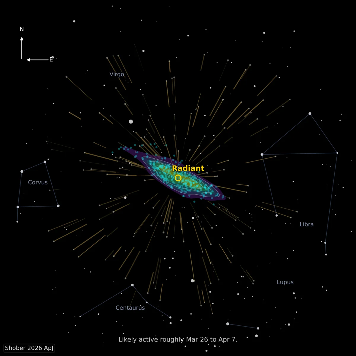
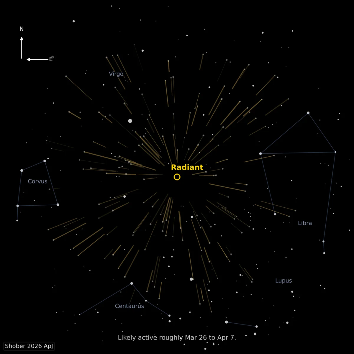
How much to smooth is the one genuinely delicate choice. Too narrow a kernel and the background inherits the very clumps you’re testing; too wide and it flattens real structure and makes everything look significant. In the 2024 paper I picked the width by cross-validation; by 2025–26 the machinery had moved to a per-dimension bandwidth chosen with the improved Sheather–Jones estimator, with the cyclic angles embedded as sine–cosine pairs so that 359° and 1° are neighbors rather than opposites.

Step 4 — Decide how loose is too loose

Once you can generate fake skies, you can ask the question that actually matters: at a given D threshold, what fraction of “matches” are coincidences? That’s the whole point of A&A 686, A130. For one specific question — which of 824 European Fireball Network fireballs belong to an established meteor shower? — the thresholds that keep false positives under 5% are:

Criterion	Threshold for <5% false positives
DN (Valsecchi)	≈ 0.15
DH (Jopek)	≈ 0.10
DSH (Southworth–Hawkins)	≈ 0.07
D′ (Drummond)	< 0.05

Those numbers belong to that dataset and that question, and nowhere else. They describe fireballs matched against known, dense showers, in a catalog of one particular size and density. Change any of that — compare meteorites with asteroids, or fireballs with each other, or use a catalog ten times larger — and the false-positive rate at a given D is a different number, and the only way to learn it is to run the null test again on that population. There is no universal threshold, and a D value quoted without its population is not a result.

Within the EFN question, traditionally people used D_SH < 0.2. That is far too generous. Applying the strict version, the genuinely shower-associated fraction converges to 150–200 fireballs, about 18–25% — against the up-to-45% previously attributed.

There’s a sting in the tail, and it’s worth quoting directly: “the meteors that meet the limiting requirement, irregardless of how low, could be spurious.” Between 6 and 11% of fireballs with D_N < 0.2 are false positives — and they are not the ones with the largest D values. You can never point at an individual pair and call it clean. You can only ever quantify the proportion.

A strict cut answers one question and spoils another

Everything above optimises purity — keeping the false-positive rate low. That is the right objective when the question is does this stream exist at all?, which is the question this page is about. It is the wrong objective once the stream is established and you want to know what it actually is: how many members, how far it spreads in solar longitude, whether it has substructure, what its real dispersion is.

For that job a tight cut is actively harmful, and not merely because it discards real members — it discards them non-randomly. You preferentially keep the tightest core, so you underestimate the stream’s extent and overestimate how compact it is, then measure its properties on the biased remnant. D-criteria trade completeness against contamination exactly this way, and Moorhead (2016) quantifies that trade for each of them. You can see the same thing in the widget above: M2026-A1’s own members have a median D_N of 0.088, so any cut tight enough to be clean keeps only its core.

If mapping the whole stream is the goal, there are better tools than a threshold:

• Cast wide, then verify independently. Link at a deliberately high threshold and confirm membership by other means — the CAMS approach of Jenniskens & Nénon (2016).
• Membership probabilities instead of a verdict. Treat the catalog as a mixture of stream and sporadic and give every meteor a probability of belonging, rather than a yes/no; Jopek & Bronikowska (2017) builds the coincidence-probability machinery that needs. Mixture models are already doing useful work on meteor data along a different axis: Hemmelgarn, Moskovitz & Vida (2026) fit a Gaussian mixture model to factor-analysed observables for 28,177 LO-CAMS meteors and recover physically meaningful groups — clustering meteoroids by what they are made of rather than by orbital similarity.
• Model the stream physically. Eject particles from the parent, integrate them forward, and ask which observed orbits the model predicts — Vaubaillon et al. (2005), Ryabova (2007), Egal et al. (2019). This is the only route that can tell you about the parts of a stream Earth never passes through.
• Measure the dispersion directly rather than inferring it from whatever survived a cut — Moorhead, Clements & Vida (2021) on radiant dispersions in GMN data.

The method follows the question. Detection wants purity; anatomy wants completeness. Reaching for a strict D threshold when the goal was the second is a common and quiet way to get a confident, biased answer.

Step 5 — Look at the whole population at once

Here is the move that makes weak streams detectable. Instead of judging pairs one at a time, count all of them: plot the number of pairs closer than D, against D, on log–log axes. This is the cumulative similarity distribution.

For a population with no streams in it, this curve is a straight line. That isn’t a convenient approximation — it’s geometry. Random points in d dimensions give N(<D) ∝ D^d, so D_N, built from four measured quantities, should give a slope near 4. Measured across six radiant catalogs in A&A 702, A36, the observed slopes are 3.75–3.88 with uncertainties of 0.21–0.30 — consistent with 4, as expected for pure chance.

A real stream breaks the line. It adds a population of very-low-D pairs that chance cannot supply, so the curve kinks upward at the small-D end. You are looking for a bend, not a number.

That was a sandbox. Below is the catalog itself — the same sizes, but the actual random draws, with whatever stream members genuinely landed in them, and a switch to take them out. At full size it is the paper’s own observed curve against its own KDE null.

The published version: the observed curve pulls away from the chance envelope under D_N ≈ 2 × 10⁻² and — crucially — stays above the band even once the reported measurement uncertainties are folded in. Of the four networks, GMN is the only one where the excess survives that test.

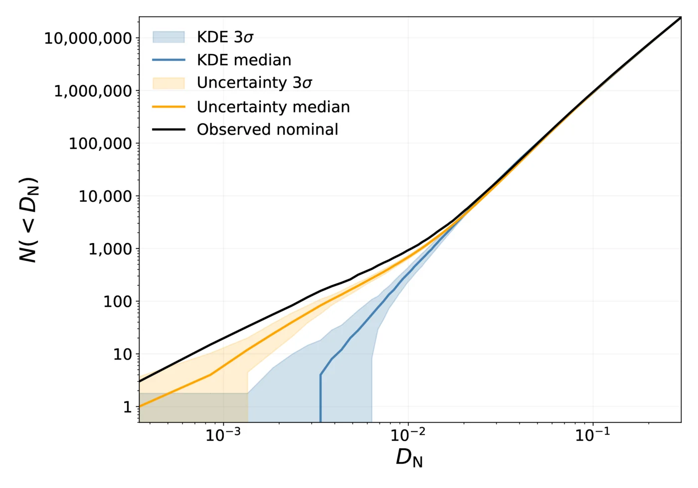
There is a physical reading of that left-hand end. A small D means two meteoroids were released from their parent with very little relative speed, so in the companion plot for D_H I put a second axis across the top converting D into an ejection velocity, calibrated by Monte Carlo — injecting particles from each observed orbit and fitting the median. On that scale the kink at D_H ≈ 10⁻² corresponds to ejections of order 100 m s⁻¹, which is the regime of genuinely recent, gentle release. Pairs below the kink are not just similar; they are too similar to have been thrown apart long ago.

Step 6 — Find out where the excess is

A bend in the cumulative curve tells you a surplus exists somewhere; it doesn’t say where. So the next step splits the sky into cells — encounter speed on one axis, date on the other — and asks, cell by cell, how many close pairs it holds against how many the null predicts. Each cell gets a z-score. Flag anything above 3σ.

Then comes the correction that most claimed detections skip. Scanning 400 cells means taking 400 chances, so a 3σ local result is not a 3σ result. The Dunn–Šidák adjustment converts a local p-value to a global one, p_global = 1 − (1 − p_local)^m, and it is brutal. Drag the slider below and watch a detection lose most of a sigma.

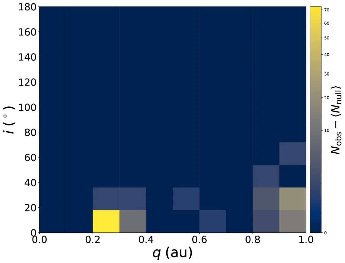
Project the meteors from the significant cells back into orbital space and the surplus resolves into one bright spot at low perihelion and low inclination.

Step 7 — Pull the members out

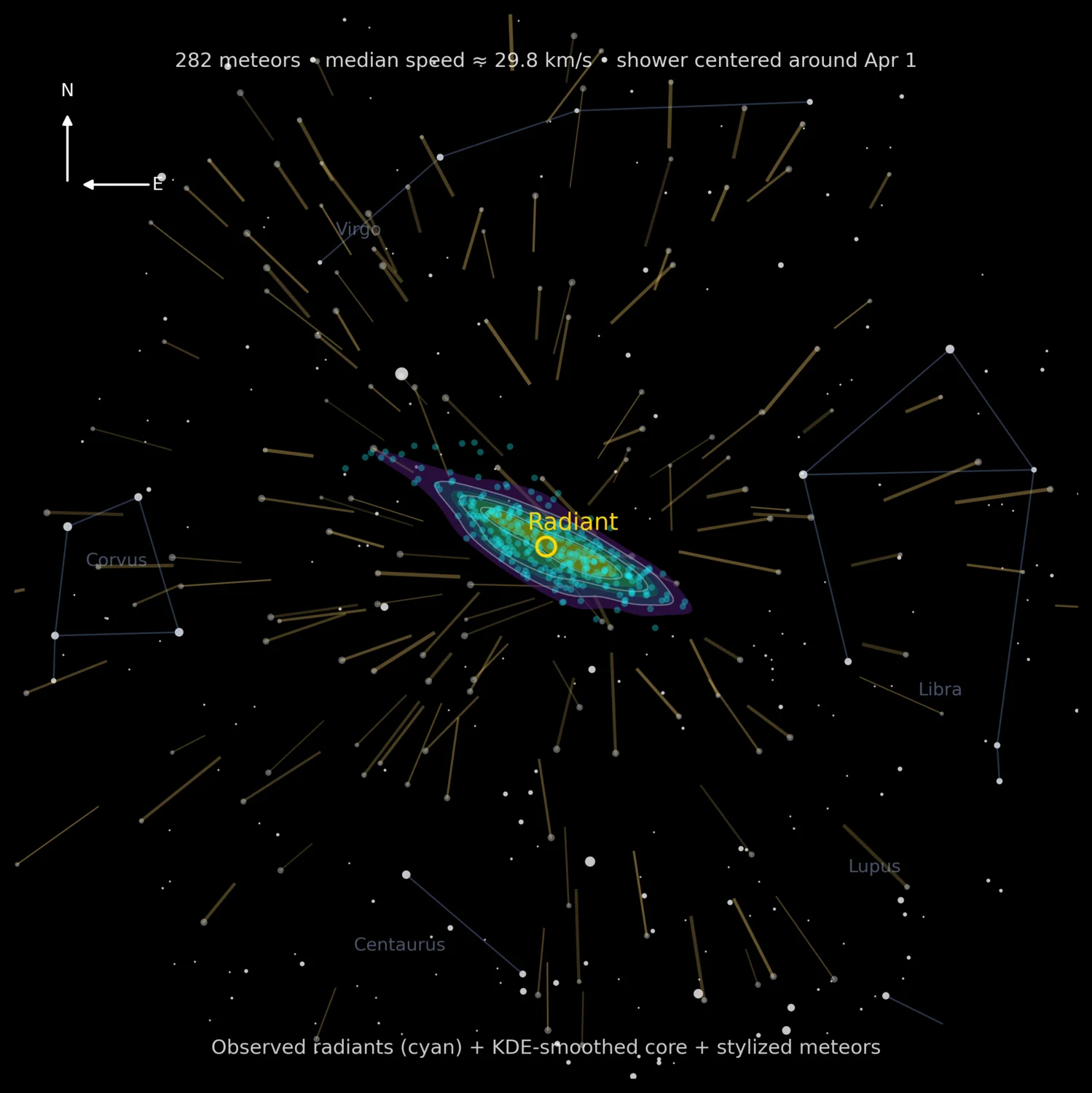
Only now, with a localized and globally corrected detection in hand, is it safe to cluster. Running DBSCAN in D_N space with ε = 0.03 and a minimum of two members yields a connected group of 282 meteors — 243 from GMN, 19 from SonotaCo, 10 from CAMS, 10 from EDMOND. Four independent networks, built and run by different teams, seeing the same thing.

What it turned out to be

The cluster is a new meteor shower, and it now carries the provisional designation M2026-A1 on the IAU Meteor Data Center working list — it appears there without an IAU number yet, which is what a working-list entry looks like before it is established. Activity in this part of the sky had been submitted once before, as candidate shower 87 Virginids (IAU #01185, code ESV), and was subsequently removed for want of evidence. This is the first time its statistical significance has been established.

Its orbit is the interesting part. Median values across the 282 members: q = 0.22 ± 0.01 au, a = 1.29 ± 0.10 au, e = 0.83 ± 0.02, i = 12.3 ± 1.8°, and a Tisserand parameter of 4.6 ± 0.3. (Those ± figures are the spread of the members, not error bars on the mean.) A Tisserand parameter that high means asteroidal, not cometary — there is no ice here to drive activity. And yet a perihelion of 0.22 au brings the parent closer to the Sun than Mercury ever gets.

That combination is what’s known as a rock comet: a body shedding debris through thermal fracture, dehydration cracking and mineral breakdown near the Sun rather than through sublimating ice. (3200) Phaethon and the Geminids are the archetype. The meteoroids’ measured strength fits — weaker than Geminids, sturdier than cometary material — consistent with a recent, thermally driven, near-Sun degradation pathway.

No parent body has been identified. It may have faded, fragmented, or come apart entirely, leaving the debris as the only evidence it was ever there. NASA’s NEO Surveyor, which is built to see exactly this kind of small, dark, low-perihelion object, is the obvious place to look next.

The results that were nothing

Most of this work returns nulls, and they matter just as much.

The same machinery, pointed at the question of whether asteroids tidally disrupted during close passes of Earth leave detectable debris families, finds nothing convincing. At most 53 meteors out of 235,271 could plausibly be attributed to such an event — an upper limit of ~2.3 × 10⁻⁴ — and they don’t cluster coherently. The long-term signature in the perihelion distribution that would confirm it is simply absent. “Some process is erasing or overwhelming the signal.”

Likewise, dozens of published claims linking specific meteorites to specific near-Earth asteroids do not survive the null test. Across 46 recovered falls and 535 candidate meteorite-dropping fireballs compared against six independent asteroid radiant catalogs, A&A 702, A36 finds no excess at all: if meteorite streams exist, they account for less than about 0.1% of falls.

They don’t cluster among themselves, either. In A&A 693, A23, 50 recovered falls, 616 probable meteorite-dropping fireballs, and 310 US Government sensor impacts all show pair counts entirely consistent with random association — no statistically significant stream in any of them, on any criterion. Their cumulative similarity curves are straight lines. The one population with a genuine excess is the telescopic near-Earth asteroid catalog, and even there the clustered fraction is at most a few percent. So when someone reports that a meteorite’s orbit is “very close” to an asteroid’s, the honest response is not how close? but out of how many? — and every time that question has been asked properly, the answer has been chance.

Why single pairs will never work

There is a hard physical limit underneath all of this, and it’s the subject of A&A 693, A23. Near-Earth space is chaotic. The Lyapunov time — the horizon beyond which two initially identical orbits diverge unpredictably — is only 60 to 200 years there. But the decoherence time, the span over which a whole stream stays recognizable against the background, is 10⁴ to 10⁵ years.

The analogy in that paper is smoke from a chimney. Individual particles start wandering apart almost immediately, driven by tiny air currents — that’s the Lyapunov time. Yet the cloud itself stays visibly a cloud for far longer as it drifts away — that’s decoherence. A stream can remain a discernible group long after its constituent members have stopped being individually traceable.

The consequence is unforgiving, and it’s the sentence I’d most like people to take away:

Any association between a specific fireball, meteorite, and asteroid, based solely on orbital similarity, is likely coincidental rather than indicative of a true physical connection.

Streams of many objects: findable. Individual parent bodies from orbits alone: not. Confirming one needs something else — composition, cosmic-ray exposure age, spectra.

Other ways people search

Cumulative similarity plus a localized excess map is what I use, but it’s one option among several. Single-neighbor linking (Lindblad 1971) grows chains of mutually similar orbits. Grouping around a mean orbit (Sekanina 1970) iterates toward a stream center. Density mapping (Welch 2001) looks for peaks directly. DBSCAN and HDBSCAN (Sugar et al. 2017; Peña-Asensio & Ferrari 2025) find dense regions without assuming a shape. Wavelet transforms are standard for radar radiant surveys. For a survey of the field, see Courtot et al. 2026.

They differ mostly in how they cluster. None of them removes the need for the null model — whichever you pick, you still have to know what chance would have handed you.

A note on the printed equations

Two of the D-criterion equations as typeset in my papers contain errors. They are typographical: the code that produced every published result uses the correct forms, so no result in any of these papers is affected. I’m noting them here because someone reimplementing a criterion from the printed page would get wrong numbers and have no way to know.

• A&A 686, A130 eqs. (18) and (20) — repeated in A&A 702, A36 eqs. (4) and (6) — print the second branch of Δξ as 2 sin((180° − φ₂ − φ₁)/2). The middle term should be 180° + φ₂ − φ₁ — a shifted difference, not a sum — as in Valsecchi, Jopek & Froeschlé (1999) eqs. (24) and (26). The sum form isn’t rotation-invariant, and it contradicts the sentence printed directly beneath it in both papers — that Δξ is small when φ₁ − φ₂ and λ₁ − λ₂ are both close to 180°, the case of two meteors meeting Earth at the two nodes of essentially the same orbit.
• A&A 686, A130 eq. (14) prints the last term of D_H as ((e_B + e_A)(2 sin(Π/2)))². The eccentricity sum should be halved: ((e_A + e_B)/2)² (2 sin(Π/2))². That is what eq. (6) for D_SH in the same paper prints, and what Courtot, Shober & Vaubaillon (2026) eq. (3) gives. As printed, the term is four times too large.

One thing that is not an error but reads like one: these papers use lowercase π for the angle between perihelia, so sin(π/2) appears in the equations. That π is an angle, not 3.14159.

The calculator above uses the correct forms, and is checked against the analysis code over several thousand cases.

Tools, data, and working together

The false-positive method has public code on Zenodo, and the 235,271-meteor dataset behind the 2026 paper is archived at doi.org/10.5281/zenodo.18664293.

The larger analysis pipeline — the cumulative-similarity engine, the four D-criteria, KDE null models with per-dimension bandwidths, the MPI pair streaming needed to get through 10¹¹ comparisons, the (U, λ☉) grid search and the clustering — is not public yet, along with the code that generates the animations on this page. If you’d like to use either, extend them, or work on this together, email me. I’d genuinely rather these got used than sat on a disk.

If you want to try the approach yourself, you need four things and none of them are exotic: a catalog of meteor orbits, a similarity criterion, a background model you trust, and the discipline to test the null before you believe the signal. The last one is the only hard part.